Also see code.
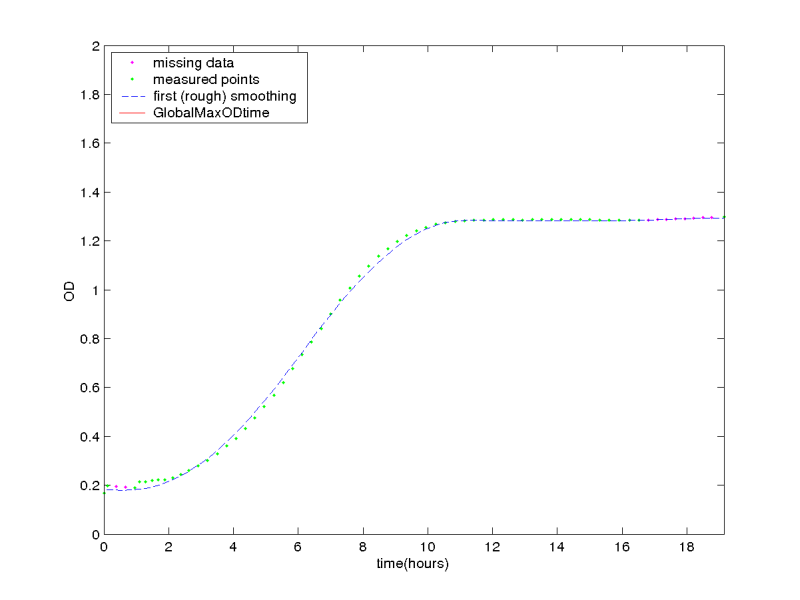
To allow comparison between the OD readings taken for different strains we model the former as continuous curves. In fitting a curve to the data we follow a data-oriented approach, whereby we approximate the curve by cubic spline polynomials rather than assuming a particular curve function (e.g. exponential curve) [Liakata08]. We proceed by applying a cycle of the following steps:
Biologically motivated indicators are calculcated automatically from the smoothed growth curves. These growth indicators include lag time, growth rate, global max od (which are widely used in biometric studies as well as other parameters such as doubling time, start, end and duration of the phase of exponential growth, the max OD reading at the end of the exponential growth phase. A series of parametric and non-parametric statistical tests are applied next to check the effect of the nutrient and that of the strain on each of the growth indicators.
Description of the curve fitting algorithm
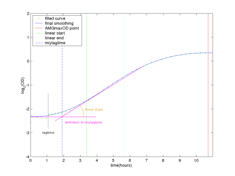
lag time is measured on the final smoothed curve. It represents the time it takes for there to be a sign of growth in the curve, taken as the point at which the first derivative of the curve exceeds a certain threshold (slopes > (0.01*max(slopes)), where slopes are the values of the first derivative. (see diagram 1 below)
miy lag time is measured on the final smoothed curve. It is the time elapsed (measured in decimal hours) between the start of OD measurements and the timepoint corresponding to the intersection between the minimum OD and the linear part of the growth curve (phase of maximum exponential growth). See description in pink, diagram 1.
miy lagtime is a standard estimation of the lag phase according to biologists. We call it miy as Mike Young introduced us to it. Even though it seems to be more accurate than lag_time the drawback is that its definition depends on the accuracy of our estimation of the phase of maximum exponential growth (linear part).
Measured on the final smoothed curve. Time point (measured in decimal hours) at which the period of maximum exponential growth (linear part) begins. (see diagram 1 below) The period of maximum exponential growth is defined as the part of the growth curve where the second derivative changes sign (from positive to negative) and the first derivative (slopes) has values within 10% of the maximum slope value. (see diagram 2 below, red crosses)
Measured on the final smoothed curve. Time point (measured in decimal hours) at which the period of maximum exponential growth (linear part) ends. (see diagram 1 below)
Meausured on the final smoothed curve. It is the duration of the period of maximum exponential growth (measured in decimal hours).
Measured on the final smoothed curve. It is the tangent of the slope of the period of maximum exponential growth (see the orange section, diagram 1). linearslope= (endlinOD-startlinOD)/(endlinear-startlinear)
Measured on the final smoothed curve. It is the max OD reading at the end of the maximum exponential growth.
Measured on the final smoothed curve. It is the timepoint (measured in decimal hours) corresponding to the maximum OD reading at the end of the maximum exponential growth. It is taken as the first point after the end of the maximum exponential growth where the slopes (first derivative) become negative or zero.
The time it takes for the cells to divide and double themselves during the period of maximum exponential growth (measured in decimal hours). It is defined in terms of the linearslope: doubletime = 1/(linearslope +.00001) (the latter is to avoid division by zero for strains that didn't grow)
Maximum optical density of the growth curve. Measured on the first raw smoothed curve.
Measured on the first raw smoothed curve. Time point at which the maximum optical density of the growth curve is achieved (measured in decimal hours). signal to noise ratio
Signal to noise ratio gives an indication of the amount of noise associated with the growth curve data. It is defined as the ratio between the range of values in the smoothcurve (max(smoothcurve)-min(smoothcurve)) divided by the average difference between the smoothed curve and a spline of the original filled curve. It is a positive number and a reliable curve should have a sn_ratio of over 100.
Is a range of values 10% either side of the maximum slope (1st derivative) of the final smoothed curve. (see green line in diagram 2 below)
Diagram 1
Diagram 2 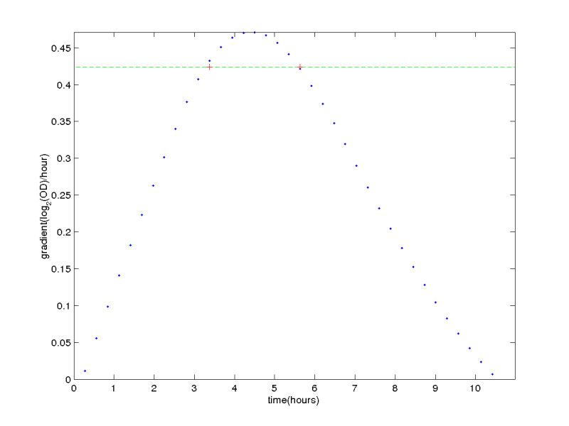
Diagram 3